Introduction to Symbolic Mathematics
Purpose:
The purpose of this experiment is to
learn how to do symbolic mathematics via Mathematica.
Equipment
and Chemicals:
A PC
running Mathematica 3.0 and a printer.
Directions:
See the instructor for directions on
how to load and run Mathematica.
Calculations:
Note in the following that all Mathematica functions are start with a capital letter,
e.g., Sin
[x], Exp [x], not sin [x] or exp [x].
Differentiation:
We can use Mathematica to take derivatives
symbolically. The basic form of the
derivative command is D[expression,var].
For example:
Example
1:
Input: D[Sin[x],x]
Output: ![]()
Example
2:
Input: Clear[k]
Input: D[Sin[k x],x]
Output: ![]()
To take the n-th derivative of f, use D[f[x],{x,n}]. To differentiate with respect to several
variables for instance, you could use D[f[x,y,z],{x,1},{y,2},{z,1}]. This computes the following fourth partial
derivative:
Example
3:
Output: ![]()
Another example is:
Example
4:
Input: D[f[x,y,z],{x,1},{y,2},{z,1}]
Output: ![]()
Notice that the superscripts which
specify the order of the partial derivative appear in the same order that the
variables are passed to the function. It
does not depend on the order in which the derivatives are specified. Thus, taking the x and y derivatives in
the opposite order gives the same result.
Example
5:
Input: D[f[x,y,z],{y,2},{x,1},{z,1}]
Output: ![]()
INTEGRATION:
Next we consider integration. Integrate[f[x],x]
returns the indefinite integral of f(x).
The arbitrary constant associated with the indefinite integral is set to
zero. Integrate[f[x],{x,xmin,xmax}]
computes the definite integral of f(x)
between xmin
and xmax. You can do a definite multiple integral using
the same syntax as for a numerical multiple integral. That is Integrate[f[x,y],{x,xmin,xmax},{y,ymin,ymax}] computes the multiple integral of f(x,y). To compute an indefinite multiple integral
you need to nest the command Integrate
as shown below.
Example
6:
Input: Integrate[Integrate[x^2
Sin[x y],x],y]
Output: ![]()
Example
7:
Input: test=Integrate[1/(2+
Output: 
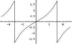
We can even use Mathematica to plot a
function. Plot[f, {x, xmin,
xmax}]
generates a plot of f as a function
of x from xmin to xmax. Here we plot the function we just calculated.
Example
8:
Input: plot1=Plot[test,{x,-5,5}];
Output:

Example
9:
Input: ![]()
Output: ![]()
As your laboratory assignment, use Mathematica to
solve the following Calculus problems. Print out your results.
Differentiation:
Calculate y’ and y’’ for each of
the following:
1. ![]()
2. ![]()
3. ![]()
Consider the function z, such that ![]() . Calculate the
partial derivatives
. Calculate the
partial derivatives
 ,
,  ,
, , and
, and  for the function
![]() .
.
Integration:
Calculate the following integrals.
1. 
2. 
3. 
4. 
5. 