Analysis of Variance
Analysis of Variance, better known as ANOVA for short, allows the researcher to compare the differences among many sample groups. Where t is for "two", the F ratio, which is the calculated value obtained from ANOVA, can handle any number of group comparisons. T testing allows us to only have two groups (experimental and control). With ANOVA, we can set up a number of experimental groups to compare with the control group. The F ratio receives its name from its founder Ronald Fisher.
For example, consider the cholesterol example we had for homework. In the homework we had two groups (Those exposed to exercise and those who were not), now we can also add in a group who is taking an experimental cholesterol-lowering medication.
The question might arise "why not just do T tests". After all, we could conduct successive t tests. If we have 3 groups, then we could test group 1 versus group 2, group 2 versus group 3, and group 1 versus group 3. Why would this not be advisable?
Because if we set alpha level to .05, we are saying that we are willing to accept a mistake 5 times out of 100, if we perform multiple t tests then aren’t we stating that we accept greater alpha levels. Of course, if we perform multiple tests there are multiple opportunities to commit an error.
ANOVA is limited in that, unlike the t test, we cannot conduct directional tests. Therefore, while the test is limited, the writing of the null hypothesis is easier to write. For example, suppose we are interested in seeing if there is a statistically significant difference between the mean shooting scores between three different shooting techniques taught to correctional officers during their academy. The null hypothesis would be written as follows:
![]()
Since we are comparing the groups all at one time, then if we set the alpha level at .05, then the alpha level stays at .05; regardless of how many groups are included in the study.
HOW ANOVA WORKS
Variance, if we think back, is a measure of the amount that all scores in a distribution vary around the mean of the distribution. A large variance value indicates a large amount of difference from the mean and a small variance value indicates very little difference from the mean of the distribution.
The question that inevitably arises when several groups of scores are being compared, is which mean a score should be compared to. After all, with t tests the answer was simple – there were two means and they were compared to each other. With ANOVA there are three or more means. So which mean do we compare with? This is where Ronald Fisher came in—he argued that the solution was to examine them all. To do this he developed a formula that would sort out the variance between the different means and then compare these variance components (hence, the name Analysis of Variance); this procedure is known as partitioning the variance.
Variance is separated into the variance between and the variance within. (Illustrate this concept on the board with an example). Between variance is the variance we want to look for because this the variance that we can attribute to our treatment effect. Within variance is variance that we cannot explain because it happens within the group (this variance is referred to as error).
POST HOC IN ANOVA
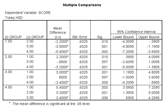
Post hoc testing allows us to go back and examine the differences between the groups in an attempt to discover where the differences lie. After all, finding a statistically significant difference in ANOVA only tells us that there is a difference we still have to figure out where the differences lie. The main thing to remember about post hoc testing is that it is only required if we find that there is a statistically significant difference. If there is not, then there is no need to continue examining the post hoc. Once we have information relating to where the differences lie, we can then make clear-cut statements about which group performed the best in the study. We will walk through a couple of these.
ASSUMPTIONS OF ANOVA
TYPES OF ANOVA
There are multiple types of ANOVA. In this course we will focus only on two of the types of ANOVA – One way ANOVA and Two way ANOVA. The only difference is that one way ANOVA deals with one independent variable and one dependent variable. A two way ANOVA deals with two independent variables and one dependent variable. The interpretation of both are similar, there is just more to remember when dealing with a two way ANOVA. We are going to work an example of each.
One Way ANOVA – here we have one independent variable and one dependent variable. For example, suppose we are interested in determining whether there is a statistically significant difference between the mean scores on an introduction to criminal justice examination when considering four course formats: a lecture class, an online class, a weekend intensive class, and a compressed video class. We enter the data into the computer and receive the following information:
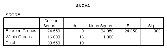
We therefore reject the null hypothesis and find that there is a statistically significant difference between the means for the various groups. Now, however, we have to examine the post hoc tests to determine where the differences lie.
To run a one way ANOVA on SPSS:
Open a data file
Analyze
Compare Means
One Way ANOVA
Move the dependent variable into the Dependent List box
Move the group variable into the factor box
Post Hoc
Put a check by Tukey
Continue
OK
Two way ANOVA – here we have two independent variables and only one dependent variable. The procedures are very similar to the one way ANOVA (they both operate the same but the calculations are drastically difference); interpretation requires a little bit more time as well, since there are two independent variables and therefore there are more hypotheses. There are three hypotheses in a two way ANOVA. For example, suppose we are wanting to examine weight loss. We take 20 individuals and we place them into two groups of ten. One group will be placed on a diet with less than 2000 calories and the other group will be placed on a diet above 2000 calories. Further, within each group 5 individuals are assigned an exercise program and the other 5 individuals are assigned to a program of no exercise. Now we have two independent variables, Exercise and Diet. The information is input into the computer and we receive the following results.
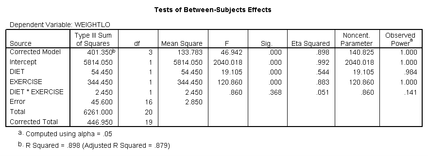
We find in examining the above tables that the null hypotheses for Diet and Exercise are both statistically significant, however, the interaction was not. Therefore we must fail to reject. There would be no post hoc here only because there was only 2 groups tested. If there were 3 then we would have conducted post hoc.
To run a Two Way ANOVA on SPSS:
Open a data file
Analyze
General Linear Model
Univariate
Move the dependent variable into the dependent variable box
Move the independent variables into the fixed factors box
Post Hoc
Move independent variables into the Post Hoc for Factors box
Check Tukey
Continue
Options
Move all available factors into the display means for box
Check Descriptive statistics, estimates of effect size, and observed power
OK